Parallel Coordinates Plot with Circular Variables

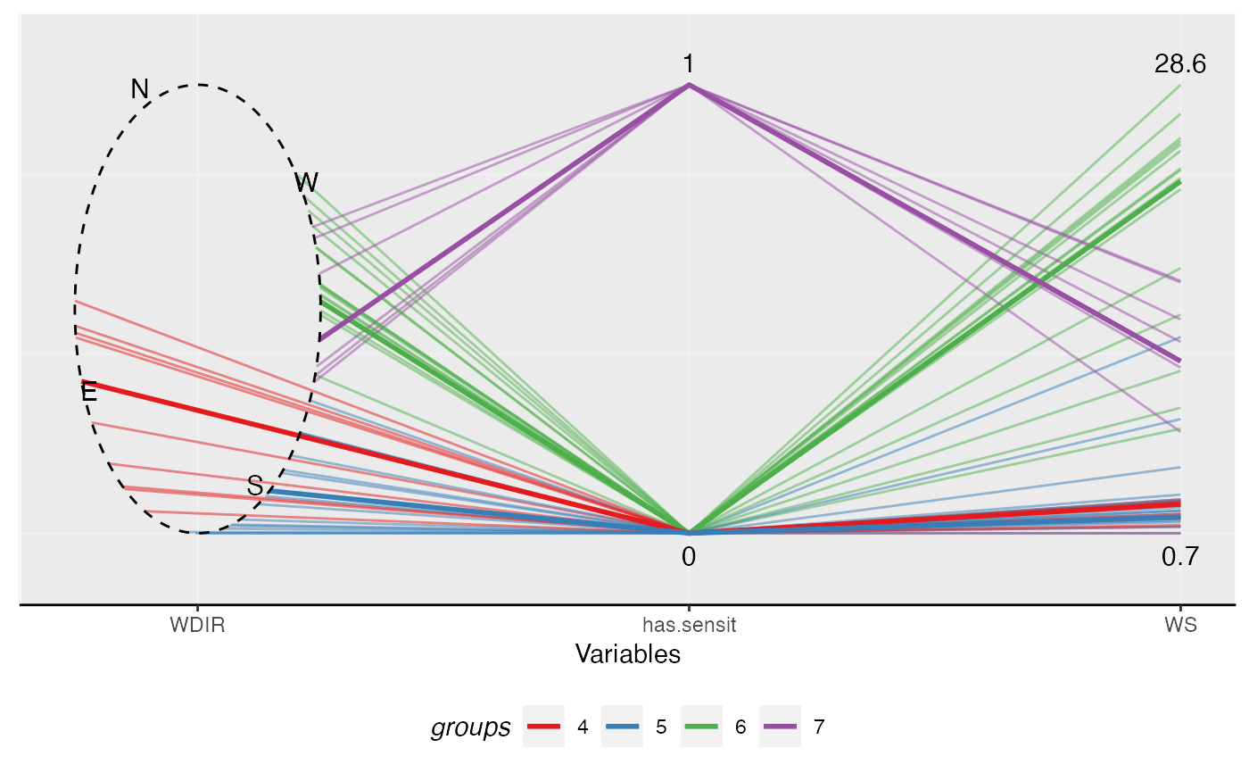
Making a parallel coordinates plot with the circular variables are plotted as ellipses. The function currently works well with data with one circular variable.

ggpcp(
  data,
  circ.var = NULL,
  is.degree = TRUE,
  rotate = 0,
  north = 0,
  cw = FALSE,
  order.appear = NULL,
  linetype = 1,
  size = 0.5,
  alpha = 0.5,
  clustering,
  medoids = NULL,
  cluster.col = NULL,
  show.medoids = FALSE,
  labelsize = 4,
  xlab = "Variables",
  ylab = NULL,
  legend.cluster = "groups"
)

Arguments

data	Data set.
circ.var	Circular variable(s) in the data set, indicated by names or index in the data set.
is.degree	Whether the unit of the circular variables is degree or not (radian). Default is TRUE.
rotate	The rotate (offset, shift) of the circular variable, in radians. Default is 0 (no rotation).
north	What value of the circular variable is labeled North. Default is 0 radian.
cw	Which direction of the circular variable is considered increasing in value, clockwise (TRUE) or counter-clockwise (FALSE). Default is TRUE.
order.appear	The order of appearance of the variables, listed by a vector of names or index. If set, length has to be equal to the number of variables in the data set.
linetype	Line type. Default is solid line. See details in vignette("ggplot2-specs").
size	Size of a line is its width in mm. Default is 0.5. See details in vignette("ggplot2-specs").
alpha	The transparency of the lines. Default is 0.1.
clustering	Cluster membership.
medoids	Vector of medoid observations of cluster. Only required when show.medoids = TRUE.
cluster.col	Color of clusters, indicating by a vector. If set, the length of this vector must be equal to the number of clusters in clustering.
show.medoids	Whether to highlight the median lines or not. Default is FALSE.
labelsize	The size of labels on the plot. Default is 4.
xlab	Labels for x-axis.
ylab	Labels for y-axis.
legend.cluster	Labels for group membership. Implemented by setting label for ggplot color aesthetics.

Value

A ggplot2 object.

Examples

# \donttest{
# Set color constant
COLOR4 <- c("#e41a1c", "#377eb8", "#4daf4a", "#984ea3")
# Reduce the size of the data for for sake of example speed
set.seed(12345)
wind_reduced <- wind_sensit_2007[sample.int(nrow(wind_sensit_2007), 50), ]

sol42007 <- MonoClust(wind_reduced, cir.var = 3, nclusters = 4)
#> Warning: binary variable(s) 1 treated as interval scaled

library(ggplot2)
ggpcp(data = wind_reduced,
      circ.var = "WDIR",
      # To improve aesthetics
      rotate = pi*3/4-0.3,
      order.appear = c("WDIR", "has.sensit", "WS"),
      alpha = 0.5,
      clustering = sol42007$membership,
      medoids = sol42007$medoids,
      cluster.col = COLOR4,
      show.medoids = TRUE) +
  theme(panel.background = element_rect(color = "white"),
        panel.border = element_rect(color = "white", fill = NA),
        panel.grid.major = element_line(color = "#f0f0f0"),
        panel.grid.minor = element_blank(),
        axis.line = element_line(color = "black"),
        legend.key = element_rect(color = NA),
        legend.position = "bottom",
        legend.direction = "horizontal",
        legend.title = element_text(face = "italic"),
        legend.justification = "center")
# }