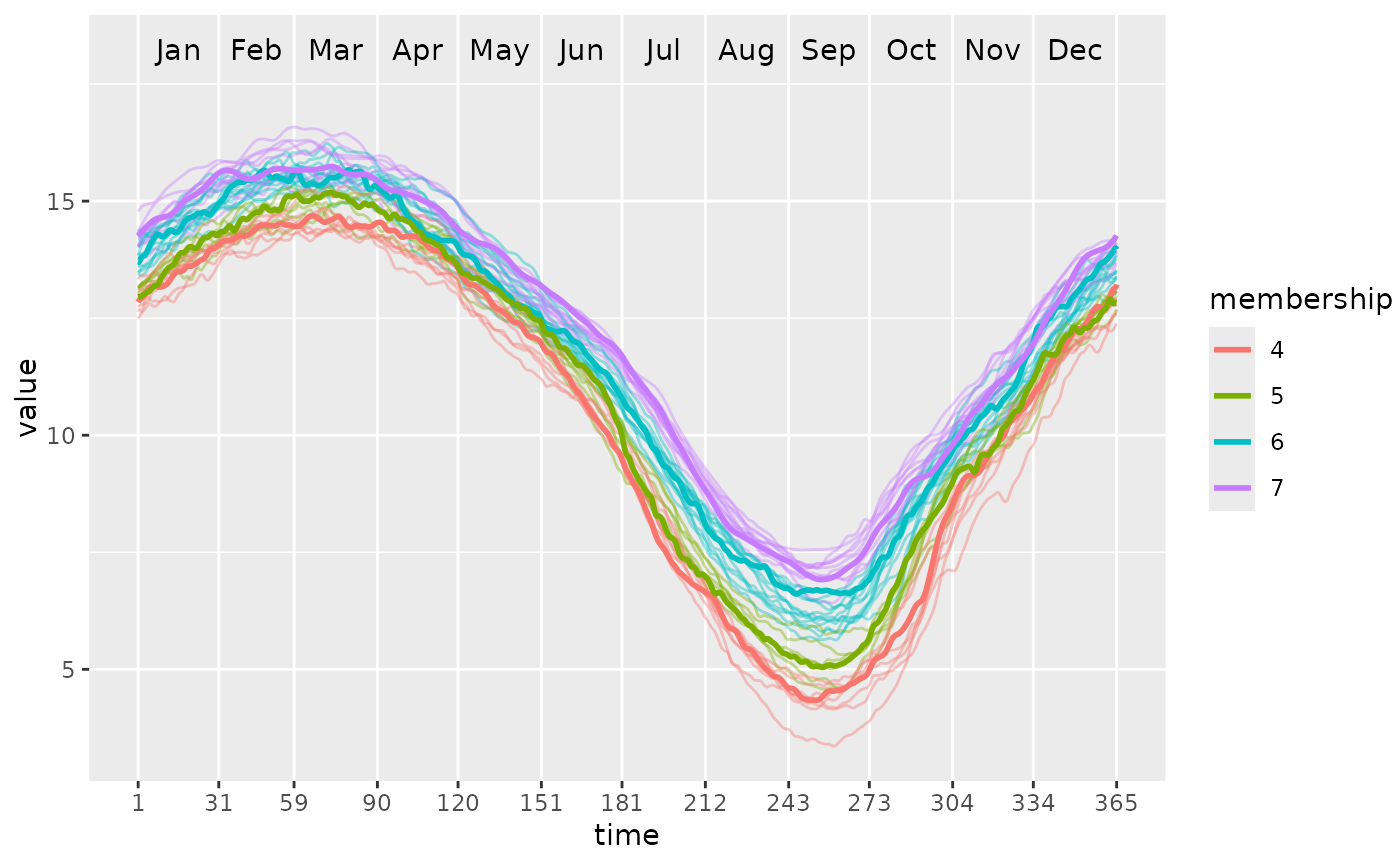
Plot the Partitioned Functional Wave by PULS

After partitioning using PULS, this function can plot the functional waves and color different clusters as well as their medoids.

Usage

ggwave(
  toclust.fd,
  intervals,
  puls.obj,
  xlab = NULL,
  ylab = NULL,
  lwd = 0.5,
  alpha = 0.4,
  lwd.med = 1
)

Arguments

toclust.fd: A functional data object (i.e., having class fd) created from fda package. See fda::fd().
intervals: A data set (or matrix) with rows are intervals and columns are the beginning and ending indexes of of the interval.
puls.obj: A PULS object as a result of PULS().
xlab: Labels for x-axis. If not provided, the labels stored in fd object will be used.
ylab: Labels for y-axis. If not provided, the labels stored in fd object will be used.
lwd: Linewidth of normal waves.
alpha: Transparency of normal waves.
lwd.med: Linewidth of medoid waves.

Value

A ggplot2 object.

Examples

# \donttest{
library(fda)

# Build a simple fd object from already smoothed smoothed_arctic
data(smoothed_arctic)
NBASIS <- 300
NORDER <- 4
y <- t(as.matrix(smoothed_arctic[, -1]))
splinebasis <- create.bspline.basis(rangeval = c(1, 365),
                                    nbasis = NBASIS,
                                    norder = NORDER)
fdParobj <- fdPar(fdobj = splinebasis,
                  Lfdobj = 2,
                  # No need for any more smoothing
                  lambda = .000001)
yfd <- smooth.basis(argvals = 1:365, y = y, fdParobj = fdParobj)

Jan <- c(1, 31); Feb <- c(31, 59); Mar <- c(59, 90)
Apr <- c(90, 120); May <- c(120, 151); Jun <- c(151, 181)
Jul <- c(181, 212); Aug <- c(212, 243); Sep <- c(243, 273)
Oct <- c(273, 304); Nov <- c(304, 334); Dec <- c(334, 365)

intervals <-
  rbind(Jan, Feb, Mar, Apr, May, Jun, Jul, Aug, Sep, Oct, Nov, Dec)

PULS4_pam <- PULS(toclust.fd = yfd$fd, intervals = intervals,
                  nclusters = 4, method = "pam")
ggwave(toclust.fd = yfd$fd, intervals = intervals, puls = PULS4_pam)

# }